The sponge that just won't saturate: radiative forcing in a hothouse Earth

Earth's beautiful glow

Teaching undergrad spectroscopy was much about theory, with a bit of lab practical, and little on critical applications. Greenhouse gases (GHGs) were covered in terms of line densities, atmospheric residence times and global warming potential (GWP), but no depth of analysis of radiative forcing, the key driver of warming and climate change. Shame on me!

So here goes with the recipe for turning those age old infrared (IR) transmission spectra of CO2 (carbon dioxide), CH4 (methane), N2O (nitrous oxide) into radiance spectra and forcing values.

Experimental CH4 ro-vib IR + Hitran x-sec

Infrared [1,2,3], is the great inbetweener (Microwave-IR-Visible) for teaching quantisation of motion in rotational and vibrational energy levels at university. Some may remember eqns like [4,5,6]

The origin of high spectral line densities for low fundamental frequencies ωe and small rotational constants B, which define ro-vibrational transition energies and spacings between them.

Great too for outreach as an intro, not only to functional group chemistry (alcohols, acids, esters), but also the greenhouse effect and the climate challenge.

With the latter, attention is given less to (grad level) quantisation and more to a qualitiaive understanding of GHGs act to trap heat from Earth and create imbalance between inbound solar and outbound IR radiation.

So what is the Earth-Sun radiation balance? It starts with blackbody radiation, the light emitted by any object at a given temperature. The intensity (or irradiance) is define by the Stefan-Boltzmann relationship [7,8] (Es in eqns below), with a strong dependence on the fourth power of the body temperature.

For the the sun of radius Rs = 695.7K km, with a surface of area, As, at a temperature Ts = 5772 K, the total power Ps, radiates into a sphere with surface of area Ad defined by the Sun to Earth distance Rd = 1.5 x 10^8 km [9]. The irradiance Ee, of Earth from the sun, known as the solar constant S0, is then the power per unit area of Earth's cross-section of radius Re. Plugging in the numbers gives...

The Solar Constant

And emitted radiation from Earth? Simply the Stefan-Boltzmann for the Earth at a surface Te = 288 K (15 oC), or....

But don't be fooled, Earth has a complex atmosphere and not all outbound radiation reaches space, not all inbound reaches Earth's surface. We have an albedo, the reflection of incoming solar from the atmosphere and surface. At around ~30% or 0.3 x 341 ~ 102  Wm-2, it makes Earth the beautiful pale blue dot it is, as seen from deep space!

Of the outbound radiation, ~40 Wm-2 (10%) radiates direct to space through the "infrared window" (10-13 microns). The remaining 356 Wm-2 is trapped by the atmosphere and adds to the warming by solar (78 Wm-2), convection (17 Wm-2) and evapo-transpiration (80 Wm-2). Hot moleules in the atmosphere then reradiate energy, some to space, some to Earth, but not evenly due to the pressure and hence concentration drop with altitude.

Figure 7.2 in IPCC, 2021: Chapter 7. [11]

Roughly, the exponential pressure profile (more later), means around 63% of molecules reside below a characterstic altitude, the scale height [10].

Thus of the total atmospheric warming 356+78+17+80 ~ 531 Wm-2, roughly 0.63 x 531 ~ 334 Wm-2 is "stored", below the scale height, while 0.37 x 531 ~ 196 Wm-2 emits freely to space.

Total outbound irradiance is then the sum of solar reflection, the IR window and atmospheric emission 102+40+196 ~ 338 Wm‑2.

Surprise! They don't balance. The in/outbound difference is small, but very real. Clear sky vs cloud cover, northern vs southern latitude differences lead to some local variation on these numbers, but with uncertainties of order 1 Wm-2, the reality is a net positive radiative forcing of 1-3 Wm-2 and warming consequences!

Lowering GHG concentrations will have effects on broadening the IR window and lowering the effective height of IR heat loss to space, with an overall effective of bringing in/outbound irradiances closer to balance.

Of course, the opposite is true as we now experience with increasing atmospheric GHG concetrations, increased forcing and increasing global temperatures.

So to the source of the problem, our GHG molecules and their spectroscopy!

CO2, CH4, and N2O are primary GHGs, and while H2O is more potent as a vapour, its variability due to precipitation keeps it out of the GHG club. Along with O3 (ozone), all these gases have absorption lines in different regions of the blackbody emission spectrum of Earth.

Spectra of primary GHGs [12] and the Planck distribution at mean surface temperature ~ 288 K

Not all light is the same, and by splitting the IR radiation from Earth into its component frequencies (energies) we get the spectrum of radiant emissions. For individual atoms/molecules spectral lines are discrete, but sum many (billions of trilliions of) atoms in a bulk object and the spectrum is continous as described by a cornerstone equation of quantum mechanics, the Planck distribution [13]...

where h = Planck constant (6.6x10^-34 J s), c = speed of light (3x10^8 m s-1) , kB = Boltzmann's constant (1.38x10^-23 J K-1) , T = blackbody temperature (K). Emissivity of Earth is close to unity (>0.95) and assumed here for simplicity.

Wavenumber is a spectroscopic unit (cm-1) of energy, the inverse of wavelength in cm, with a consant of proportionality c, to convert to frequency or hc, to energy. The Stefan-Boltzmann relation derives from integration of the distribution over all wavelengths.

Molecules in the atmosphere put a dent in (attenuates) the Earth's radiance, the size of which depends on the line intensity (extinction ε) at each frequency (wavenumber) in the molecules absorption band, the concentration of GHGs through the atmosphere and temperature variation with altitude.

Beer-Lambert Law

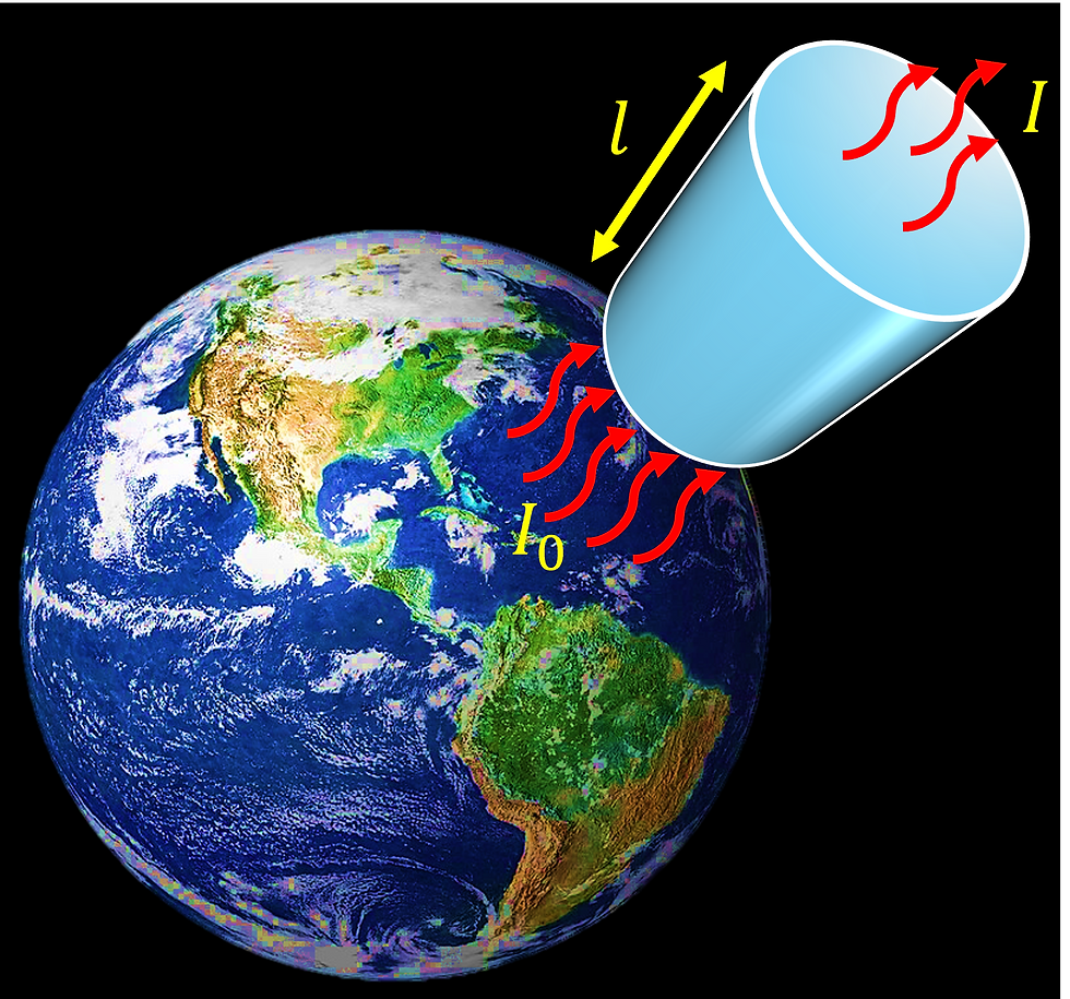
For light of intensity I0, passing through gas column of length L, at gas concentration C, with molar exctinction ε, the transmitted light intensity I, is given by the Beer-Lambert Law [14,15]

and the light absorbed is simply I0 - I.

The concentration of gases through the atmosphere is not constant but decreases with altitude. Climb Everest and you soon run low on oxygen!

Gravity pulls the mass of molecules toward the surface creating an exponentially decreasing pressure P, with height from the surface h, as described by the barometric formula and characterised by the scale height, H and surface pressure P0 [10]. For well mixed gases in the lower atmosphere a "mean", abundance weighted mass, m ~ N2(0.79 x 28) + O2(0.21 x 32) ~ 0.029 kg and effective temperature, Ta ~ 254 K, defines the pressure profile.

atmospheric GHG concentrations [16]

The pressure profile is converted to concentration via the ideal gas equation for a surface temperature, Ts ~ 288 K. Ozone differs in profile, peaking around ~ 8 ppm at ~ 35 km through UV photolysis of oxygen and the interplay between a decreasing concentration of O2 with altitude, but increasing intensity of solar UV.

Climate change consequences [17]

Rising CO2 ppm since the industrial revolution around 1750 is the primary source of radiative forcing and a chain of climate consequences; temperatures not seen in over 100 000 years and extreme events, floods, heatwaves, drought, crop failures, all expected to rise in risk by multiples at a predicted 3 oC warming by the end of the century.

Back to business. Like concenctration, temperature through the atmosphere is not constant, but its profile is more complex and defines four distinct layers (International Standard Atmosphere [10]), the troposphere (0 ~ 11 km), stratosphere (11 ~ 50 km), mesophere (50 ~ 85 km) and thermosphere (85 ~ space).

Atmospheric Pressure / Temperature Profile

The boundary (pause) between each layer, is defined by a strong inversion of the lapse rate = -dT/dh, the -ve of the temperature gradient [10].

The result is a zig-zag temperature profile, with lapse rates, 6.5 K/km from surface to the tropopause, -2.1 K/km to the stratopause and 2.3 K/km to the mesopause.

At a certain altitude, IR absorptions turn to transmissions as concentration drops, marking the effective emission height at which IR escapes to space. This height then maps to an effective emission temperature on the atmospheric profile.

Between absorption bands, the effective emission temperature is just the surface temperature of the Earth that defines the Planck distribution, since there are no IR absorbing transitions and heat is transmitted from the surface at h = 0. For IR lines wihin each GHG band, emission heights and temperatures correspond to the point at which transmision equals absorption according to the Beer-Lambert Law.

The Beer-Lambert Law and concentration profile combine to give the transmission intensity dependent on concentration C0, altitude height h, path length L (characterised by 1/C0.ε), and extinction coefficient ε. For each slab of atmosphere of thickness L, there is a height h, at which the intensity of light transmitted equals that absorbed by the gas, i.e. I = I0 - I and the ratio, I /I0 = 0.5.

CO2 (bend mode) efffective emission heights & temperatures (grey 0.01 cm-1, red 1 cm-1)

We can now derive an analytic approximation for the effective emission height, above which there is net transmission of IR to space, and below which net absorption leads to warming of the atmosphere and Earth..

Since the extinction is a function of wavelength ε(λ), across each band of spectral lines, there is a corresponding "spectrum" of effective emission heights, h(λ) and temperatures T(λ), mapped according to the warming profile of the atmosphere, T(h).

Substitution of the spectrum T(λ) for each GHG into the Planck distribution B(λ, T ) then gives the spectral radiance of the Earth and atmosphere, accounting for IR absorption from our GHGs.

Individual GHG contributions to the radiance of Earth and sum total

Radiative forcing, is the metric for the extent to which solar irradiance is effectively enhanced (positive) or reduced (negative) by different mechansims, including ice/aerosol reflectivity (albedo) and land use (forest/farmed/urban).

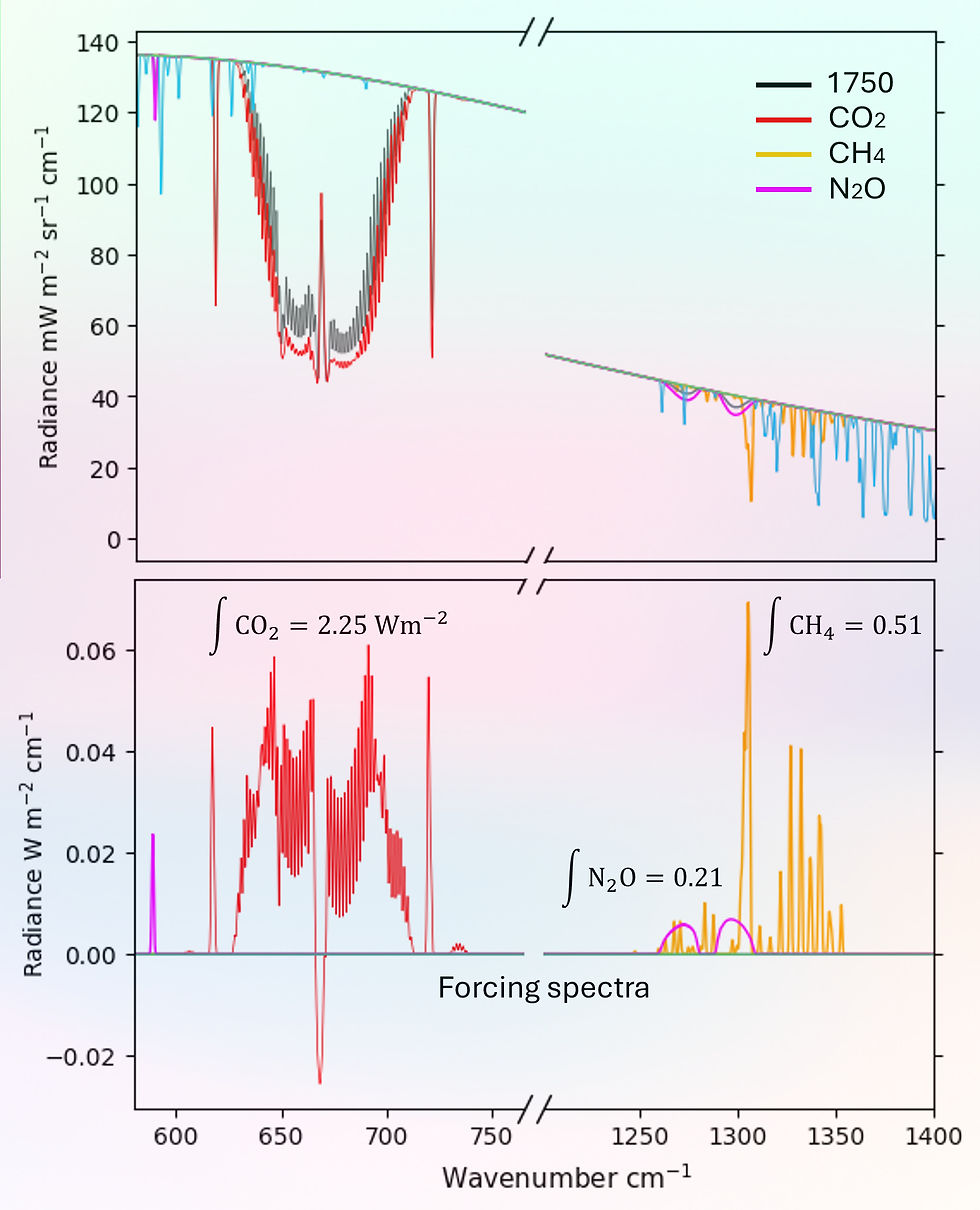
For GHGs forcing can now be derived from the difference in the radiance spectra arising from changes in atmospheric concentrations (ppm). Integration of the difference spectrum then gives the total change in radiance, the radiative forcing, e.g. for a change from pre-industrial ppm (1750) to present day levels.

Radiance spectra for 1750 and 2025 GHG ppms, difference spectra and integrated forcings

One last step! Emission from each point on Earth's surface is Lambertian and follows the cosine law that states, the radiant intensity along a line of sight from an ideal diffuse radiator is proportional to the cosine of the angle between the line and the radiating surface [14].

It simply adds a factor π, by integrating over the solid angle (steradian, sr) element

converting the sum over the difference spectrum (Wm-2sr-1) to an intensity (W m-2) of the radiative forcing.

From values of 1750 ppms to present (2025) for the main GHGs (see table), the model generates radiative forcings, CO2 ~ 2.25 Wm-2, CH4 ~ 0.51 Wm-2 and N2O ~ 0.21 Wm-2. The values strongly reflect the relative concentrations of the gases in the atmosphere, and fall close to those reported elsewhere [18].

CO2 is like a sponge, absorbing IR so efficiently that it is well and truly saturated at band centre (Q branch ~ 667 cm-1), and only transitions in the (P & R) band branches are responsible for changes in the radiance spectra and net radiative forcing.

Stratospheric cooling stripes (1979-2024) added 2025 [19] to Ed Hawkin's 2018 warming stripes

Saturation pushes emission heights deeper into the stratosphere, where gas concentrations are low, the free path of IR photons is high and molecular collisions, that can redistribute energy, are few. So molecules are free to emit IR to space.

As heights increase with ppm, increasing free paths between collisions and IR recapture, allow more molecules to radiate freely to space, resulting in net negative forcing and cooling of the stratosphere.

More interesting is the trend in radiative forcing with increasing ppm (from 1750 levels). For CO2, proxy records (e.g. ices cores) place ppms during glacial periods at 2.5X lower than current levels, around 190 ppm with forcing -2.2 Wm-2 lower than today, and a doubling from pre-industrial levels to 560 ppm, gives the climate sensitivity of 2X CO2 ~ 16.5 - 12.9 ~ 3.6 Wm-2.

Radiance in the spectral band regions of CO2, CH4 and N2O and trends in radiative forcing

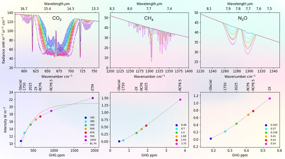
As CO2 levels rise IR transitions in the (P & R) branchs of the band saturate, and only weaker lines deep in the wings still have capacity to absorb. The band broadens and total absorption (area under the dip) increases with a saturating trend.

Current levels of 430 ppm sit around 15/19 ~ 80% the level expected to be reached by the end of the century (2100) in a "business as usual", IPCC RCP8.5 (Representatitive Concentration Pathway) scenario [20].

RFs: a = 2025, b = 2X 1750, c = RCP6, d = RCP8.5 [19], CH4 & N2O glacial ppm scaled as per CO2 (190/280)

RCP indices refer to the radiative forcing (6 & 8.5 Wm-2) arising from effects that can be mapped to carbon dioxide concentration equivalents (CO2e). In this case both RCP6 and 8.5 are reproduced well by the model (b) = 4.5 + 0.4 + 0.5 ~ 5.4 Wm-2 and (c) = 6 + 1.4 + 0.6 ~ 8 Wm-2, given that forcings from changes in ice, cloud, aerosol, and land use are not accounted for.

By 2300 CO2 in RCP8.5 is expected to approach 2000 ppm [19], close to the Eocene Thermal Maximum (ETM) around 50M years past [21]. Radiative forcing from CO2 then reaches 22.4 - 12.9 ~ 9.4 Wm-2, but signficantly saturation, in accordance with simple Beer-Lambert absorption, is never reached due to continued broadening and the increasing rise of weak transitions in the band branches.

While CO2 and temperatures have been 5X higher during periods of "hothouse" Earth, including the Cretaceous period when dinos walked the Earth, it's worth noting evidence that these giants were mesothermic [22]; somewhere between cold- and warm-blooded, and like reptiles today, suited to warmer climes.

Mammals at this time were small, and during the Eocene, an evolutionary period of dwarfing in larger species occured to adapt to higher temperatures, through increased surface area (to volume) and efficient heat loss [23]. And for sure there were no sapiens, only a very remote relative, Purgatorius mckeeveri [24].

Temp vs CO2 vs Population

60M years later and CO2 today is now at levels not seen for over 100 000 years in the last interglacial period, a time when human populations were a only few hundred thousand [25] compared to the 8 billion+ now required to adapt to a warming world.

Back to forcings! CH4, N2O differ in trend from CO2, remaining in a "linear" regime over the ppm range from current to RCP 8.5 or 2X levels. That is, forcing is directly proportional to GHG concentration with no sign of a saturation limit at high ppm.

While ppms and hence forcings remain a fraction for CO2, it is notable that forcings per ppm are signficantly stronger, CO2 = 2.25/150 ~ 0.015 vs CH4 = 0.51/1.24 ~ 0.41 vs N2O = 0.21/0.07 ~ 3 Wm-2 ppm-1.

Forcings relative to CO2, CH4 at 0.41/0.015 ~ 27X and N2O at 3/0.015 ~ 200X now correlated well with (100 yr) Global Warming Potentials (GWP) of the gases [25], a key indicator of the relative potency of each as GHG to trap IR and induce warming!

The effect of forcings on the extent of warming and surface temperatures is complicated by climate feedback effects on ice/cloud albedo, lapse rates, carbon and water cycles. Moreover, the slow uptake of heat by oceans, effectively reduces radiate forcing by an estimated FO = 0.42 W m-2. Feedback effects are then accounted for in a climate sensitivity parameter

where is S = 1.8 oC and ΔT is the temperature change for a total forcing ΔF, given a sensitivity to doubling CO2 of F2X. The model 2X sensitivity of 3.6 Wm-2 and current forcing of 2.25 + 0.55 + 0.21 ~ 3 Wm-2 then gives a temperature anomoly of ΔT = 1.8 x (2.97 - 0.42) / 3.6 ~ 1.3 oC and rising! With all the consequences that an energised atmosphere, warming oceans, melting ice and a heat stressed biosphere brings.

Sources and sinks for GHGs are many, natural, geological and biogical, as well as engineered and anthropoligical in origin. Since climate stability is strongly coupled to atmospheric GHGs through radiative forcing, control of GHG cycles from sources to sink is critical to avoid future tipping points; in precipitation patterns of rainforests and monsoons, ocean circulation and acidification, polar and gacial ice loss, boreal permafrost stability, freshwater scarcity and biodiversity.

Reducing GHG emissions and crucially our dependence on fossil fuels, is essential to setting Earth on a path to a more sustainble climate. Avoiding emissions via capture at source, enhancing drawdown to sinks, or compensating for warming through solar, emissivity and albedo management, may just help Earth on that path. How fast we scale solutions, natural or engineered, will determine where exactly where that pathway ends.

[1] Herschel, William (1800) XIV. Experiments on the refrangibility of the invisible rays of the sun. Phil. Trans. R. Soc.90284–292 http://doi.org/10.1098/rstl.1800.0015

[2] Foote, Unice (1856). Circumstances affecting the heat of the Sun's rays, p382 Art. XXXI, AAAS

[3] Tyndal, John. (1872) On Radiation Through The Earth's Atmosphere in Contributions in Molecular Physics, Phil. Trans.

[4] Sommerfiled, Arnold (1923), Atomic structure and spectral lines, E. P. Button & Co., Inc., New York.

[5] Pauling, L, Wilson, E. B. (1935). Introduction to Quantum Mechanics with Applications to Chemistry. McGraw Hill Book Company Inc.

[6] Coblentz, William W. (1905). Investigations of Infra-Red Spectra. Carnegie Institution of Washington.

[7] Stefan, Josef (1879) über die Beziehung zwischen der Wärmestrahlung und der Temperatur. Sitzungsberichte der Kaiserlichen Akademie der Wissenschaften in Wien, Vol. 79, Aus der k.k. Hof-und Staatsdruckerei, 391-428.

[8] Boltzmann, Ludwig (1884) Ableitung des Stefan'schen Gesetzes, betreffend die Abhängigkeit der Wärmestrahlung von der Temperatur aus der electromagnetischen Lichttheorie. https://doi.org/10.1002/andp.18842580616.

[9] https://nssdc.gsfc.nasa.gov/planetary/factsheet/sunfact.html

[10] US Standard Atmosphere 1976, Washington, D.C. ISO International Standard Atmosphere. ISO 2533:1975

[11] Figure 7.2 in IPCC, 2021: Chapter 7. In: Climate Change 2021: The Physical Science Basis. Contribution of Working Group I to the Sixth Assessment Report of the Intergovernmental Panel on Climate Change. doi: 10.1017/9781009157896.009

[12] https://hitran.org/hapi/; R.V. Kochanov, I.E. Gordon, L.S. Rothman, P. Wcislo, C. Hill, J.S. Wilzewski, HITRAN Application Programming Interface (HAPI): A comprehensive approach to working with spectroscopic data, J. Quant. Spectrosc. Radiat. Transfer 177, 15-30 (2016). https://doi.org/10.1016/j.jqsrt.2016.03.005

[13] Planck, Max (1900). Zur Theorie des Gesetzes der Energieverteilung im Normalspectrum. Verhandlungen der Deutschen Physikalischen Gesellschaft. 2: 237–245.

[14] Lambert, Johann Heinrich (1760). Photometria, sive de mensura et gradibus luminis, colorum et umbrae. Augustae Vindelicorum : sumptibus viduae Eberhardi Klett typis Chistophori Petri Detleffsen

[15] Beer, August (1852). Bestimmung der Absorption des rothen Lichts in farbigen Flüssigkeiten. Annalen der Physik und Chemie (in German). 162 (5): 78.

[16] https://www.climatelevels.org/

[17] Wim Thiery et al., Intergenerational inequities in exposure to climate extremes. Science374,158-160(2021). DOI:10.1126/science.abi7339

[18] https://www.ipcc.ch/report/ar6/wg1/figures/chapter-7/figure-7-6

[19] Hawkins, E., and Coauthors, 2025: Warming Stripes Spark Climate Conversations: From the Ocean to the Stratosphere. Bull. Amer. Meteor. Soc., 106, E964–E970, https://doi.org/10.1175/BAMS-D-24-0212.1.

[20] https://www.ipcc.ch/site/assets/uploads/2017/09/WG1AR5_AnnexII_FINAL.pdf

[21] https://projects.noc.ac.uk/jmodels/documentation/paleocene-eocene-thermal-maximum

[22] John M. Grady et al. Evidence for mesothermy in dinosaurs. Science344,1268-1272(2014).DOI:10.1126/science.1253143

[23] D'Ambrosia AR, et al. Repetitive mammalian dwarfing during ancient greenhouse warming events. Sci Adv. 2017 Mar 15;3(3):e1601430. doi: 10.1126/sciadv.1601430.

[24] https://www.nationalgeographic.com/science/article/did-ancient-primates-walk-alongside-dinosaurs-new-evidence-backs-up-theory

[25] Per Sjödin, et al. Resequencing Data Provide No Evidence for a Human Bottleneck in Africa during the Penultimate Glacial Period, Molecular Biology and Evolution, Volume 29, Issue 7, July 2012, Pages 1851–1860, https://doi.org/10.1093/molbev/mss061

[26] https://www.ipcc.ch/report/ar6/wg1/downloads/report/IPCC_AR6_WGI_Chapter07_SM.pdf

*Links accessed 29/7/2025