The Milankovitch cycles: from ancient astronomy to a climate chronicle

Updated: Jul 1

As sure as night follows day, we know the Earth rotates on its axis. Clocks spring forward, fall back around the equinox, and the solstice that marks the longest day of Summer and shortest in Winter, tells us the Earth orbits the sun.
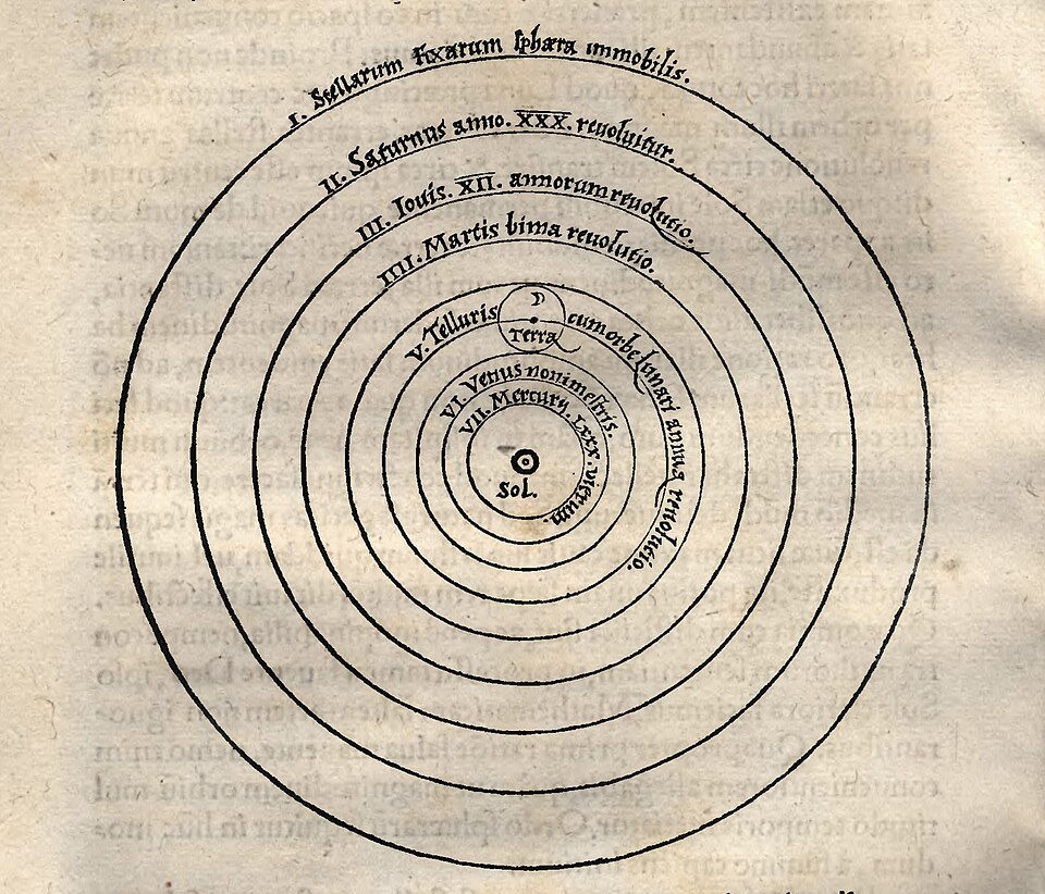
Of course that was only made obvious when Copernicus (1543) [1], from celestial observation, placed the sun at the centre of the solar system. Before that, sunrise after the dark of night, fruitful summers and freezing winters were the hands of the gods!
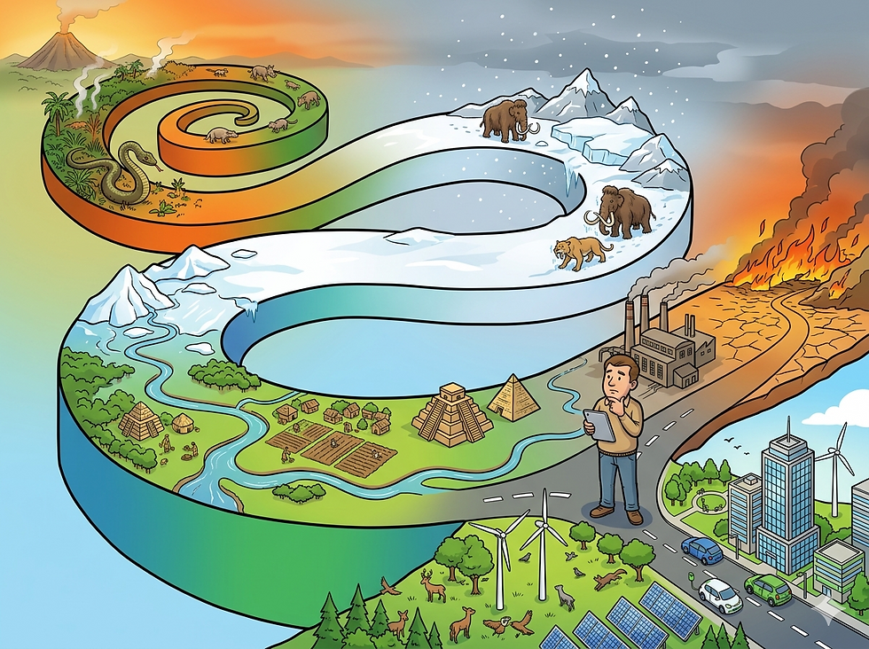
Less obvious are the subtle peroidic changes in these cycles, known as the Milankovitch cycles. Their effects on Earth's climate are dramatic, ultimately dictacting the timing of ice ages and warmer interglacial periods. Luckily, these cycles operate on long geological time scales of many thousands of years.
This dive aims to sit somewhere between qualitative descriptions and the rigourous mechanics of the Milankovitch cycles. A bit of history and just enough maths to shine a light on the science behind our Earth's evolving climate.
From spinning tops to wobble boards
The view of Earth spinning on an axis was first conjectured by Greek astronomers of Pythogoros and Platonic camps, Philopaus and Heraclides [C4th BC], in a challenge to the ancient picture of the heavens spinning about a fixed Earth, as painted by Aristotle.

Obliquity, or axial tilt was first measured by Pytheas of Marseille (350 BC) [2], using the trigonometry of shadows cast by a gnomon (upright of a sundial) at his name place. At the Summer solstice noon, Pytheas quoted a gnomon height to shadow length ratio 209/600, giving the intermal ray-to-earth, projection angle
By alternate angles, this gives the latitude of the location with respect to the orbital plane, but not to the equator.
The same measurement at the equinox then gives the latitude from the equator directly where it intersects the orbital plane. The gnomon now casts a longer shadow, with a height to length ratio round 0.94 (~209/222), a projection angle, and hence latitiude of 44.3°.
The difference gives an obliquity of 24.1°, a value larger than today's tilt of 23.5°, but close to that 2000+ years past, given the obliquity is now known to have been in decline over the last 10000 years. A difference of < 0.6° from the shadow of stick, remarkable!
Axial Precession, the slow roll of Earth's axis around a fixed pole, like a kids spinning top, was first identified by Hipparchus of Rhodes (190 BC).
The plane of the equator necessarily wobbles in concert with the axis, such that the position of the equinox on Earth's orbit, shifts slowly over time. The constellations at the March equinox are seen to creep westward with this precession of the equinox.

Hipparchus (129 BC) compared location of the star Spica in the northern night sky with records of Timocharis (293 BC), and concluded the stars made a longitudinal shift around 1° in a century, a full revolution in 36000 years.
Despite such understanding of the heavens, the geocentric view of Ptolemy's Algemist (150 AD) [3] prevailed for centuries, where day, night and seasons were dictated by motions of the celestial bodies about a central Earth (geo = Earth, helios = Sun in greek). The Algemist provides the only records of Hipparchus and development of the epicycle-deferent (sphere-on-sphere) model of celestial motions.
Translations of the Indian text Surya Siddhanta (800 AD) suggest refinement of the "trepidation" of the equinoxes with 54° shift-and-return over a 7200 year cycle, or axial precession of 54" pa (2X54X3600/7200) and period 24000 years [4].
Tables of Ulugh Beg (1347), refine star displacements to 1° in 70 years, an precession rate of 51.4" pa and period of 25 200 years. Translations of the Persion astronomers text indicate a first to measure the obliquity at 23.5° [5].
Copernicus (1543) [1] later showed the precession of the equinox to be variable about a mean 50.2" pa, close to modern measurements of an axial precssion period around 26000 years.
Around the same time Fracastoro (1538) [6] appears the first to acknowledge a north-to-south, latitudinal shift in the precession of the equinoxes from a change in obliquity.
Aspsidal Precession, the wobble the orbital plane, was first identified by Hipparchus through observed anomalie in the Moon's apogee (farthest point from Earth) [3]. Ancient, Babylonian records were used to show it took 126007 days for the Luna eclipse to return to the same position in the night sky, within which time 4573 anomaly returns and 4612 orbits of Earth were noted.
Hipparchus recognised the difference arising from motion of the Moon's apsides (axes of orbit). The anomoly and orbital periods, 27.55 days (126007/4573) and 27.32, respectively, determine the precession period (T) from the "beat" frequency (ω) of the two cycles.
Modern measurements place the Moon's precession period at 8.85 years, while Earth's small, slow aspidal precession (relative its axial precession), was not identified until the precision of the 19th Century.
Primitive heliocentric views of the early Pythagorean astronomers were ultimately substantiated by Copernicus [1], who proposed that motions of the planets could only be explained by placing the sun at the centre of their orbits. Not until the following century, with Galileo's (1610) [7] invention of the astronomical telescope, was this view and motions of the five known planets Mercury, Venus, Mars, Jupter, Saturn confirmed [8].
At the same time Kepler published the first mathematical laws governing planetary motion (1609, 1619) [9], based on accurate sextant measurements of Mars' orbit by Tycho (Brahe) (1574) [10]. Newton (1687) followed up by identifying gravity as the force driving the motion [11].

Kepler's key finding? Triangles made from lines connecting the sun to the arc swept by a planet over a fixed time, are all equal regardless of distance between sun and planet. The planet must orbit faster at points closer to the sun than points farther from the sun, with a the crucial conclusion, that the orbit must be ellipitcal.
Eccentricity is defined by the semi-major and semi-minor axes of the elliptic orbit, governs the distance of closest approach to the sun, the perihelion and furthest, the aphelion, and determines the lengths of seasons. Kepler's value of 0.018 is today measured at 0.0167.

A calculated enlightenment
By C18th, accuracy of instruments and calculus accelerated discovery of new motions, with 3rd Astronomer Royal, Bradley [1747], first to identify a nutation of the obliquity; an 18 year, 9" wobble in the rotation axis from the pull of the moon [12]. His measurements allowed later derviations of an overall decline in axial tilt of around 0.45" pa [13]. Limits on the tilt came later.
Lagrange and Laplace (1766-1784) performed the first calculations of the six planetary orbits including "three body" interactions, between the planets themselves and the sun [14]. A planet's motion is then coupled to all others, forcing periodic changes in orbital inclination and the longitude of its node (pivot point), the eccentricity and longitude of the perihelion (point of closest approach).
The legacy? By treating eccentricity (and other periodic elements) as a vector changing in amplitude and direction over time, the Cartesian components (h and k) could be solved, each as trigonmetric series with amplitudes (α), frequencies (𝑔) and phases (β) defined by the strength of (gravitational) coupling between planets and its rate of change as planets orbit to and from each other.
Importantly changes in eccentricity were found to arise from changes in the semi-minor axes of the ellipitic orbit, while the semi-major axis remained invariant.
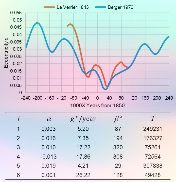
Uranus, discovered at his time by Herschel (1781) [15], was ultimately included in orbital calculations of Le Verrier (1843) that revealed (mass) corrected an eccentricity max and min of 0.06 and 0.003, respectively. Le Verrier (1848) went on to predict the existence Neptune, from irregularities observed in the orbit of Uranus [17].
Refined apsidal and axial precession rates of 11.66" pa (T = 360X3600/11.66 ~ 111150 years) and 50.1" pa (T = 25868 years) were reported, respectively by L.B. Francoeur (1812) and Delambre (1817) and Adhémar (1842) recognised the sourjon times combined for an overall "climate" precession period of 21000 years (360X3600/61.67) [18,19,20].
Calculations of the orbital eccentricity, inclination and longitude of the perihelion were subsequently corrected by Stockwell (1873), with the inclusion of all 8 planets in his celestial calcs [21].
By the 20th century, Pilgrim (1904) completed calculations on all secular pertubations (long term changes) in Earth's orbital properties, over extended periods (-1000000 to +40000 years), to reveal min & max of the obliquity of 22.1° and 24.5°, respectively [22].
With the current 23.5° obliquity near-midway and decreasing at a mean rate around 0.42" pa, the obliquity period is ~ 41000 years (2X(24.5-22.1)*3600/0.42).
From ice-age to nice-age & back again
![The Milankovitch cycles: past and future orbital elements & resulting insolation Q. Data generated from Laskar (La2004)[27]](https://static.wixstatic.com/media/40e0b0_d159500f421b408b890572e0e98fb227~mv2.jpg/v1/fill/w_785,h_987,al_c,q_85,enc_avif,quality_auto/40e0b0_d159500f421b408b890572e0e98fb227~mv2.jpg)
Milankovitch (1920) was the first to calculate changes in the insolation from a over 600K years before 1800, from the most accurate values of eccentricity, obliquity and precession at the time [23,24,25].
A 100 kiloyear period on the eccentricity revealed in the Milkankovitch cycles was was confirmed in a +/-5 million year projection by Berger (1976) and a final 405 kiloyear modulation was found superposed in calculations of Laskar (2010) extending back 50 million years [27].
The 100K cycle is seen in the mean rate of secular frequencies given by Berger (fig), while the gravitational pull of Venus and Jupiter on Earth's orbit, give rise to the 405K beat period from the difference in frequencies.
Finally in a full circle moment, location of the shortest distance from Earth to sun, the longitude of the perihelion, is defined with respect to the "first point of Aries", set by Hipparchus (130 BC) at the March equinox [28].

In the Earth centred view of the time, the sidereal year started here at a geocentric longitude of 0°. As the sun moved counterclockwise, the north entered summer around 90°, reached the autumn equinox near 180° and the winter solstice about 270°, where the south approaches the height of summer when Earth is closest to the sun, the perihelion.
Today, precession of the equinox at 50.1" pa has moved this first point ~30° west from Aries to Pisces in over 2000 years (50.1*(2026+130)/3600).
And the heliocentric system now flips the first point 180° such that the perihelion resides around 270-180 ~ 90°.
The equinox lands around March 20 (19 to 21), while perihelion occurs around January 3 (2 to 5), a difference of 76 days or 75° (76X360/365). Perihelion is then 360-75 ~ 285° and 105° in geocentric and heliocentric frames, respectively. A mean anomaly is applied varying between +/- 1.915°, as a sine dependent on the number of Julian calendar days after 2000 (26X365.25 + 2451545) and currently -1.88° [29]. The final longitude of the perihelion is then 105-1.88 ~ 103°.
That's it, the orbital elements defining the Milankovitch cycles are covered and collated in Table 1 below!
Cycle | Today | Max | Min | Period |
Slow 𝑒 | 0.0167 | 0.012 | -0.012 | 405000 |
Fast 𝑒 | 0.0167 | 0.058 | 0.005 | 100000 |
Obliquity ϵ | 23.4 | 24.5 | 22.1 | 41000 |
Perihelion (apsidal) | 103 | 0 | 360 | 112000 |
Equinox (axial) | First Point in Pisces moves to Aquarias by 2600 | 26000 | ||
Climate cycle ϖ | Summer solstice aligned with perihelion in 1249 | 21000 | ||
Table 1
Shedding light on our sun driven climate
So how do these orbital elements and the periods over which they change lead to the climate cycles, from ice ages to warm interglacial periods, that we see printed in the geological history of Earth?
The ancients looked to the sun gods. From Helios (Greece) and Sol (Norse) in Europe, to Ra (Egypt) in Africa, from Mithra (Persia), Syrus (Hindu), Xihe (China), Amaterusa (Japan) across asia, to Kinich Ahau (Mayan) and Inta (Inca) in the Americas, the sun has been worshipped for bringing light, warmth, life, harvests.
The amount of warming the sun brings depends on the earth-sun distance, with Herschel (1832) the first to recognise that the heat received from the sun would diminish with a decreasing eccentricity of earth's orbit [30].
The heat is inversely dependent on mean earth-sun distance (strictly the square, Lambert (1760)[31]) over a revolution. As the minor axis increases and earth's orbit becomes more circular with decreasing eccentricity, so the mean distance increases and total heat decreases.
The inverse square dependence on earth-sun distance gives a current 7% difference in heating between perihelion (shortest) and aphelion (longest), but as high as 25% and low as 2%, as the eccentricity cycles between max and min limits over 100K year timescales.
Insolation, the total solar energy received at the top of Earth's atmosphere per unit area and time, was first determined by Pouillet (1838)[32] from the temperature change of a fixed container of water exposed to the sun (the pyrheliometer) with extrapolation to the top of the atmosphere assuming exponential attenuation (as per Bougeur(1729)[33]).
Measured then at 1.7366 calories/cm2/min ~ 1211 W/m2 (4.184 J per cal), the solar constant is now measured by satellite at a mean of 1361 W/m2 and varying by only 0.1% over the 11 year sunspot cycle.
The solar constant then allows calculation of insolation at any point across the Earth and its variation across seasons (an orbit of the sun) and long term, through the 21 kiloyear precessions of the equinox, 41 kiloyear cycles of obliquity and 100+ kiloyear changes in eccentricty.
Simple geometry gets you so far, but the projection of a 2D disc of illumination on a 3D spherical earth, ultimately requires some complex derivation.

In a toy model (see fig), the curvature of the Earth can be thought as "spreading" the solar consant, S0, over an increasing projected area with increasing latitude.
For a latitude ϕ and obliquity ϵ, the irradiance is reduced by cos(ϕ +/- ϵ) at aphelion/perihelion.
The total insolation then depends on the length of day, the fraction of a 24hr (2π) rotation spent exposed to the sun.
Tilt of the rotation axis makes this half a rotation +/- an arc length east and west that depends on tilt ϵ and increases from 0 at a latitude matching the tilt (12hr day) and π at latitudes above ϕ = π/2 - ϵ (24hr sunlight) and below ϕ = -π/2 + ϵ (no sunrise).
Between aphelion and perhelion, the arc lengths are further modulated by the ecliptic longtiude, θ, locating the time of year on Earth's orbit. Approaching the equinoxes (θ = 0, π), where day-night lengths are equal, the arcs reduce to 0 as sinθ, leaving the half arc and 12hr day.
Finally the insolation is ultimately modulated by the inverse square of the Earth-sun distance RE with resepct to the orbital mean R0 to which the solar constant applies.
In practice the length of day is determined from integration of the solar zenith angle, Θ, between hour angles, +/- h0, representing sunrise and sunset.
The zenith angle is equivalent to that between a perpendicular to the Earth surface and the direction of suns rays and derived from the spherical law of cosines.
Since the perpendicular depends on the latitude ϕ, and the direction of the sun depends on its declination δ and hour angle, h, in the day, so these are found in the cosine expression.
The mismatch between orbital and axial precessions adds a phase, between "first point in Aries" (θ = 0) , at the spring equinox and perihelion, as defined by the longitude of the latter, ϖ.
The limits on the hour angles depend, in the same way as the toy model, on latitude, ϕ, and obliquity, ϵ, with modulation by the ecliptic longitude, θ. So again, at full tilt toward the sun, the high arctic never sleeps (maximum insolation) and the antarctic never sees sunrise (zero insolation).
Integration between limits gives the insolation

For current orbital elements, 𝑒=0.0167, ϵ=23.4°, ϖ=103°, the contour map of the daily insolation (W/m2) over the year (0 < θ < 360°), from the spring equinox (θ=0), shows the expected pattern of solar heat with only a small north-south asymmetry in peak solar due to eccentricity; the southern summer being at perihelion, north at aphelion.
Given the eccentricity, obliquity and precession change with time, so the insolation will vary accordingly.
The Milankovitch Cycles revealed
Milankovitch identifed that the large land mass in the northern hemisphere, would be more responsive to changes insolation, through a lower heat capacity and faster land-air heat exchange than the ocean that fills the south.
Then at a latitude, ϕ = 65°N and summer solstice, θ = 90°, the hour angle aproaches h0 ~ π, and for a small eccentricity, 𝑒 << 1 and obliquity, sinϵ ~ ϵ, the insolation reduces to
where the orbital elements are strictly functions of time as they vary over their respective periods and the dependency of insolation on the key components 𝑒(t), sinϖ(t) and ϵ(t), as seen in Milankovitch-type analyses (fig above), is made clear.

So what? How's this help understand long term changes in climate of the past and climate change of the future.
Ice cores provide a best reference for Earth temperatures, extending over 400K years past (Vostock [34]).
Analysis of the last two ice ages, ending with interglacial warming, around -20K year, shows generally good correlation between solar heating of north (Q at 65°N and the temperatue anomly (ΔT from the 1850-1900 mean).
Associations are observed between the short initial cycle of rapid warming, cooling and warming (25K years) and the large peak-to-trough amplitudes in the insolation that follows precession.
Warming is then correlated with shorter, but hotter summers where the solstice aligns with perihelion, while cooling occurs during longer, but cooler summers, as precession brings the solstice in alignment with aphelion.
Duration of the ice-age (100K year) and a slower and deeper decline in temperatures trends with the reduction in eccentricity, with low warming-cooling cycles (40K years) matching obliquity.
Temperature swings appear larger and faster at high eccentricity (-225K years of the 405K cycle) and the current period relative stability and slow cooling is expected to persist while eccentricity decreases to its minimum in around 20K years.
Currently the north tilts toward the sun at aphelion, for long, warm summers, and away at perihelion, for short, cool winters. In 13000 years of the 21K year precession cycle, the north will tilt away from the sun at aphelion, for long, freezing winters and at perihelion, short, intense summers.
The mechanism by which the climate tips into an ice age is not well understood. Early theories of Adhémar (1842), based on precession, and Croll (1864), adding effects of eccentricity on the changing lengths of seasons, landed on long cold winters at aphelion as the trigger for glaciation [20, 35]. Observations of "arctic cricle" snow lines by Buch (1800), Forbes (1853) and Murphy (1869), drew conclusions the advance of the snow line followed from longer, cooler summers [36].
Milankovitch showed that, where precession brings the summer solstice in alignment with aphelion during periods of peak in eccentricity and falling obliquity, the slow orbit far from the sun, and lower angle of solar projection combine to make summers sufficiently cool and long to prevent polar ice melt.

Time spent at aphelion is inversely dependent on speed at the turn point. Then from conversation of angular momentum at aphelion and perihelion, the ratio of time spent at these extrema is simply the ratio of their distances (Table 2).
Thus at maximum eccentricity, the summer at aphelion lasts 158/141 ~ 1.12X longer than winter; an extra 11 days (0.12X365/2.12) compared to just a 5 day (152/147 ~ 1.03X, 0.03*365/2.03) difference today, and less than 2 days at minimum eccentricity.
Eccentricity Limit | 𝑒 | Semi-major a Mkm | Perihelion rp Mkm | Aphelion ra Mkm |
Max | 0.057 | 149.597 | 141.070 | 158.124 |
Now | 0.0167 | 149.597 | 147.099 | 152.095 |
Min | 0.005 | 149.597 | 148.849 | 150.345 |
Table 2
A minimum insolation of around 430 Wm-2 (-120K & -230K yrs) is reached when obliquity dips to 22.1° and a maximum near 580 Wm-2 when precession aligns the summer solstice with perihelion (ϖ = 90) and obliquity is maxed out.
The matrix of solar irradiance and the "normalised" product of irradiance x summer to winter lengths ratio (Table 3), for the eccentricity, obliquity and precession extremes (summer at aphelion ϖ = 270° & perihelion ϖ = 90°), highlights the key role that obliquity plays in the large swings in solar heating that control long term climate changes.
Changes in insolation due to eccentricity and precession of summer between aphelion and perihelion are normalised by changes in season length, leaving the extent of Earth's tilt on its axis, the obliquity as the standout element. The central conclusion of Milankovitch!
ϖ | 𝑒 | ϵ 24.5° | ϵ 22.1° | summer: winter | ϵ 24.5° | ϵ 22.1° |
270 | 0.05 | 472 | 426 | 1.11 | 521 | 470 |
0.005 | 519 | 468 | 1.01 | 524 | 473 | |
90 | 0.05 | 577 | £520 | 0.90 | 522 | 471 |
0.005 | 529 | 478 | 0.99 | 524 | 473 |
Table 3
From climate proxies to Fourier frequencies
Geological and paleoclimate records play a founding role in the origins of the astro view of periodic climate change, ice age and interglacial cycles.
From boulders found far from their bedrock origins in the Alps [Schimper (1835), Agissiz (1838)], to oxygen isotope stages (OIS) found in deep ocean sediments [Emiliani (1954)] and GHG gas content in Vostok ice cores [Barnola (1987)], geologists, biologists and paleontologists, have looked to explain different proxies for historic climate status [37-39].
In particular charges in O(18):O(16) isotope rato (δ18O) in sediments containing carbonates (CaCO3) from ancient benthic foraminifera shells (single cell organisms) and in the water (H2O) of ice cores, have strong correlations with ocean and atmospheric temperature through mechanisms with a common origin.
Lighter H2O(16) evaporates more readily than the heavier O18 isotopomer, but a heavier H2O(18) precipitates preferentially over its counterpart. This largely follows from the fraction of molecules with sufficient speed to form vapour, decreasing with mass in accordance with the Maxwell-Boltzmann distribution as exp(-mv2/2kT) [40].
Thus in warmer waters near the equator δ18O concentrates as H2O(16) evaporates, and is depleted in water vapour moving away from the tropics, as rains remove H2O(18). Precipitation over the poles is sufficiently depleted in O(18) to exhibit negative δ18O ratios compared to standards (the Vienna Standard Mean Ocean Water).
In a cooling atmosphere CO2 sinks, the heavier O(18) isotopomer more than O(16), and in a cooling ocean the gas and carbonate ion have increased solubilty. Availability of O(18) in carbonate is then enhanced for benthic foram to sequester in shells and δ18O rises as ocean temperatures drop (+0.22 per mill rise per 1°C fall).
The deviation in benthic δ18O measured in parts per thousand (per mill) is converted to temperatures using the empirical relationship of Epstein and Urey et. al (1953) (T = 16.5 - 4.3δ + 0.14δ^2, σ = +/-0.6°C) [41].
The 100K year cycle of the mid-to-late Pleistocene epoch (11K - 1M years past) are evident in both ice and sediment records, but are other periodicities hidden in the noise?

The Fourier transform [42], a cornerstone of signal processing, is used to convert a time series signal f(t) to a spectrum of frequencies F(ν), where a signal is decomposed into a series sine and cosine functions via the transform
For the simple signals solutions can be short, singular functions (a pulse tranforms to sinc), but the power of the process lies in the extraction of key frequencies that make up "noisy" data.

Applied to benthic δ18O records the Fourier spectrum reveals peak amplitudes at decreasing frequencies 0.0456, 0.024, 0.0099 (per kiloyears) the inverse of which correspond closely to the 21000, 41000 and 100000 year cycles of climate precession, obliquity and eccentricity.
The core frequencies and corresponding phases can now be used to give a basic reconstruction of the "astronomical" model of the periodic variations in orbital elements and insolation that map to the proxy signal.
Substituting these fequencies, phases into the reduced expression for insolation, along with amplitudes for the eccentricity and obliquity, from their maxima and minima (Table 1), generates a crude but clear reproduction of the elements controlling the climates cycles reflected in the benthic foram, δ18O, proxy signal.
Importantly, superposition of the eccentricity and precession produce the large amplitude fluctuations that correlate with large swings from interglacial δ18O "lows" associated warming climates, to isotope highs in cooling cycles.

Periods of decreasing eccentricity and obliquity tend to drive higher levels of δ18O, which correspond to deeper cooling and extended ice ages.
So what of the current climate, the influence of insolation and the Milankovitch cycles?
Making sense with toy models
A closer look at the transition from the depths of the last ice-age (-30K to -11K years) to the holocene (-11K to present), we see a lag between insolation and temperature proxies, most notably δ18O records rise as insolation falls with obliquity after post glacial warming (> -10K).
Lags and phase differences are expected from inertia in the response of land, ocean and atmosphere to changes in solar warming, due to differences in heat capacities and exchange rates between these systems.
Divergence between insolation and global surface temperatures (GST) can be reconciled to an extent via the earth-sun energy balance, which is modulated through solar absorption and scatter by atmospheric gases, land and sea mass, as well as reflection and the re-emission of radiation.
The interplay between these components and their affects on Earth's climate are complex and heavy, numerical computation of highly-coupled, heat and fluid dynamics to reveal cause and affect beyond just correlations [43]. However, insight can be gained from simple physical models.
Albedo, the fraction of reflected solar, plays a key role in the transition from snowball-Earth of the ice-age to the blue planet of our interglacial age. Snow and ice are highly reflective, with high albedo (0.9 - 0.7) compared to open water and land (0.03 - 0.2) and the extent of ice cover depends strongly on temperature, as we see from polar-ice loss and sea-level rise with global warming [44, 45, 46].
The atmosphere also adds to albedo (0.15-0.25) through scatter from gases, aerosols and clouds, as well as absorbing around 30% of incoming solar across spectral bands of H2O, ozone (O3) and CO2 in the UV, visible and near to mid-infrared.
A simple model uses historic sea level records to estimate the extent of ice cover and hence albedo from present values. Until recent declines with warming, ice has covered around 21 million km2 [45] or ~ 3-4% [47] of Earth's surface and albedo (a) averages around a ~ 30% [44].
At the base of last ice-age, sea levels were up to 120 m [46] below the present rising trend. Around 40% of the sea level rise can be attributed to expansion as waters warmed [48]. Assuming the remaning 60% of water volume define by this depth and ocean area, as 70% of Earth's surface, is redistributed as ~1 km thick ice [49], cover was around (2.6+2.1)/2.1 ~ 2.2X that of the today, around 9% of Earth's surface.
Ice depth would not be constant over the snowball to warm Earth transition, but would likely have followed a rapid thinning that reflects sea level rise, just at a 10X scale (+1 km ice down to 0 v -0.1 km sea up to 0).
![Sea level [46], ice depth & cover, -ve albedo RF, +ve GHG RFs & net sum contribution](https://static.wixstatic.com/media/40e0b0_4b830d5120a643ba8f3dfd5420089ffe~mv2.jpg/v1/fill/w_781,h_833,al_c,q_85,enc_avif,quality_auto/40e0b0_4b830d5120a643ba8f3dfd5420089ffe~mv2.jpg)
The small cover but high reflectance of ice/snow, means total albedo from varies around 10%, a ~ 0.33 to 0.30, from ice-age to present.
Reflection of solar reduces irradiance and heating at Earths surface, contributing to a negative radiative forcing (RF), which varies as the product of insolation and albedo (Qice).
The major greenhouse gases (GHGs), CO2, CH4, N2O contribute positive RF through by trapping heat that would otherwise radiate to space. Absolute heat (QGHG) is dependent on atmospheric pressure records and the absorption spectra of individual GHGs (see post on Radiative Forcing).
Water vapour adds around 32 Wm-2 of heat trapping, with H2O equally reducing incoming solar by 30% (along with ozone and CO2). Increased vapour pressure and +ve (infrared) forcing due to temperature rise is somewhat balanced by -ve (visible-NIR) forcing from solar absorption.
![Insolation (@65N, black), net with -ve RF from ice cover (blue), net with +RF from GHG, temperature reconstructions (green & orange) [51] & temperature anomaly (magenta) from net solar heating](https://static.wixstatic.com/media/40e0b0_77d83e49c16d47a681697fabe2c98be8~mv2.jpg/v1/fill/w_756,h_686,al_c,q_85,enc_avif,quality_auto/40e0b0_77d83e49c16d47a681697fabe2c98be8~mv2.jpg)
Net irradiance raising the global surface temperature (GST) is then the sum of all contributions, reduced insolation due to atmospheric absorption, reflected heat from albedo and trapped heat from GHGs. At around pre-industrial numbers add to around 0.7X467 - 139 + 14 + 32 ~ 234 W m-2.
Surface temperature is estimated from the Stefan-Boltzmann relationship between temperature T, and the radiant intensity Q, of a perfect black body emitter, and the emissivity ε, of Earth compared to the black body radiator [50].
While the Earth, land, sea and ice, is a near-perfect emitter (ε > 0.9), atmospheric absorption prevents thermal radiation escaping to space and the effective emissivity is reduced to ε ~ 0.6 [51].
Applying the toy model using sea level records to determine ice volume (km3), redistributed ice cover (km2) and change in albedo across the late ice-age to holocene period (-25K to present), reproduces the temperature anomoly records (vs 1850-1900 mean) remarkably well [52].
Temperature highs around the -6K years, the holocene climate optimum (HCO), run a little hotter than proxy reconstructions, and lows at the depths of the ice-age are lower than some records.
But with inputs to the model derived simply from literature without fitting or optimisation, the model works well to elucidate the basic physics and principle components that govern climate change.
The caveat! There's nothing new to see here. Models of this kind will used in the various reconstructions of temperature profiles from proxy data (δ18O, ice-core CO2, etc), so good alignment is not unexpected.
The aim then? A long stroll through the history and science behind our Earth's evolving climate (as per intro), an ode to the giants of astronomy and climatology, a primer for action on the key drivers of our current climate trajectory.
The take aways...
Simple physical models provide clear quantitative insights!
Solar cannot account for current trends in global warming.
Cooling, not warming would be expected from the down trend in insolation.
Even accounting for loss of ice and hence albedo, net heating from solar at Earth's surface trends down.
Insolation is the dominant driver of the transition from ice-age to the holocene climate optimum (HCO) and slow cooling up to the 19th century.
Albedo and -ve forcing from changes in ice cover dominates the overall "damping" of insolation and net irradiance of Earth's surface.
GHGs add near-constant forcing over the period of transition out of the ice-age.
But since the industrial revolution, rapidly rising levels of GHGs (1750) has driven the 1.5C uptick in GST, with recent snow and ice-loss playing a minor but non-negligiable roles.
CO2 remains the dominant GHG in radiative forcing and spiking temperatures in 2026!
Key climate controls to dial down warming:
Reduced GHGs - renewables, electrification, waste reduction/recycling, carbon dioxide removals, regenerative farming.
Enhanced albedo - re-icing the polar caps, cool (white) roofs & asphalt, SRM and stratospheric aerosol injection.
Enhanced emissivity - cirrus-cloud thinning, passive cooling through the IR window (8-14 micron).
[3] Ptolemy https://classicalliberalarts.com/resources/PTOLEMY_ALMAGEST_ENGLISH.pdf; G.J..Toomer p. 175
[4] The Surya Siddhanta https://archive.org/details/TranslationOfTheSuryaSiddhanta/page/n169/mode/2up
[12] Bradley nutation https://royalsocietypublishing.org/rstl/article-split/45/485/1/25976/I-A-letter-to-the-Right-honourable-George-Earl-of
[13] Obliquity rotation https://articles.adsabs.harvard.edu//full/1840MmRAS..11...73P/0000073.000.html
[14] Lagrange & Laplace https://arxiv.org/pdf/1209.5996
[15] Herschel https://makingscience.royalsociety.org/items/l-and-p_7_192/paper-of-a-comet-uranus-seen-on-13-march-by-william-herschel?page=1
[16] Le Verrier eccentricities https://babel.hathitrust.org/cgi/pt?id=mdp.39015065119771&seq=468
[17] Le Verrier Uranus https://gallica.bnf.fr/ark:/12148/bpt6k9609947k/f9.item.texteImage
[20] Adhémar Le https://babel.hathitrust.org/cgi/pt?id=nyp.33433090749718&seq=30
[23] Milankovitch review https://cp.copernicus.org/articles/17/1727/2021/
[24] Milkanovitch 1920 book review https://projecteuclid.org/journalArticle/Download?urlId=bams%2F1183485705
[25] Milkanovitch 1941 Canon review https://scispace.com/pdf/the-astronomic-theory-of-climatic-changes-of-milutin-4dmeska4d6.pdf
[27] Laskar 2010 https://www.aanda.org/articles/aa/pdf/2011/08/aa16836-11.pdf; https://ssp.imcce.fr/insola/earth/online/earth/online/index.php
[28] First point of Aries https://www.glyphweb.com/esky/concepts/firstpointofaries.html
[29] Perihelion anomaly https://aa.usno.navy.mil/faq/sun_approx
[30] Herschel solar https://bibdig.museogalileo.it/tecanew/opera?bid=965219&seq=5
[32] Poulliet solar constant https://gallica.bnf.fr/ark:/12148/bpt6k95017r/f12.item.r=M%C3%A9moire+sur+la+chaleur+solaire,+sur+les+pouvoirs+rayonnants+et+absorbants+de+l'air+atmosph%C3%A9rique+et+sur+la+temp%C3%A9rature+de+l'espace.langFR
[33] Bougeur attenuation https://archive.org/details/UFIE003101_TO0324_PNI-2703_000000/page/n191/mode/2up
[36] Buch, Forbes, Murphy https://hgss.copernicus.org/articles/13/23/2022/
[37] Agassiz vs Schimper https://www.jstor.org/stable/25101263?seq=1
[39] Barnola, J., Raynaud, D., Korotkevich, Y. et al. Vostok ice core provides 160,000-year record of atmospheric CO2. Nature 329, 408–414 (1987). https://doi.org/10.1038/329408a0
[40] Maxwell-Boltzmann https://www.mdpi.com/1099-4300/17/4/1971; https://sites.pitt.edu/~jdnorton/teaching/2559_Therm_Stat_Mech/docs/Maxwell_1860.pdf
[41] Epstein et al. https://pubs.geoscienceworld.org/gsa/gsabulletin/article-abstract/64/11/1315/4537/REVISED-CARBONATE-WATER-ISOTOPIC-TEMPERATURE-SCALE?redirectedFrom=fulltext
[43] Climate models https://wcrp-cmip.org/ref-launch-at-cmip2026/; https://gmd.copernicus.org/articles/19/2627/2026/
[45] Ice cover km2 https://www.ncei.noaa.gov/access/monitoring/monthly-report/global-snow/202601#seaice
[46] Berends et al https://cp.copernicus.org/articles/17/361/2021/
[47] Ice cover % https://www.usgs.gov/faqs/how-does-present-glacier-extent-and-sea-level-compare-extent-glaciers-and-global-sea-level
[48] Expansion https://www.climate.gov/news-features/understanding-climate/climate-change-global-sea-level
[49] Ice thickness https://www.science.org/doi/10.1126/science.265.5169.195; https://www.antarcticglaciers.org/glacial-geology/laurentide-ice-sheet/laurentide-ice-sheet-at-the-last-glacial-maximum/; https://www.annualreviews.org/content/journals/10.1146/annurev.earth.32.082503.144359
[50] Stefan-Boltzmann https://babel.hathitrust.org/cgi/pt?id=uc1.a0002763670&view=2up&seq=306
[51] Emissivity Fig 7.2 https://www.ipcc.ch/report/ar6/wg1/downloads/report/IPCC_AR6_WGI_Chapter07.pdf
[52] McKay https://cp.copernicus.org/articles/18/911/2022/; Nick McKay. (2022). nickmckay/past-and-future-warming-comparison-figure: Climate of the past resubmission (resubmission). Zenodo. https://doi.org/10.5281/zenodo.5842209
*Links accessed 18/06/2026